FFT

A DFT and FFT TUTORIAL

A DFT is a "Discrete Fourier Transform". An FFT is a "Fast Fourier Transform". An FFT is a DFT, but is much faster for calculations. The whole point of the FFT is speed in calculating a DFT.

The Basic Idea

<< Home Next >>

A Fourier Transform converts a wave in the time domain to the frequency domain.

Note, for a full discussion of the Fourier Series and Fourier Transform that are the foundation of the DFT and FFT, see the Superposition Principle, Fourier Series, Fourier Transform Tutorial.
Every wave has one or more frequencies and amplitudes in it. An example is a sound wave. If someone speaks, whistles, plays an instrument, etc., to generate a sound wave, then any sample of that sound wave has a set of frequencies with amplitudes that describe that wave.
According to the mathematician Joseph Fourier, you can take a set of sine waves of different amplitudes and frequencies and sum them together to equal any wave form. These component sine waves each have a frequency and amplitude. A plot of frequency versus magnitude (amplitude) on an x-y graph of these sine wave components is a frequency spectrum, or frequency domain, plot. See Diagram 1, below.

An inverse Fourier Transform converts the frequency domain components back into the original time wave.

You can reassemble the time wave from the frequency components using the Inverse Fourier Transform. The inverse Fourier won't be discussed here, but after learning the Fourier the Inverse is very easy to learn, because the math is almost identical. Using the Fourier and Inverse Fourier together, not only can you reassemble the original wave, you can also change the time wave by altering its frequency components. You can add them, remove them, or tweak their values. This is a powerful method by which to change the character of the time wave.
A DFT is a "Discrete Fourier Transform". An FFT is a "Fast Fourier Transform". The IDFT below is"Inverse DFT" and IFFT is "Inverse FFT". A DFT is a Fourier that transforms a discrete number of samples of a time wave and converts them into a frequency spectrum. However, calculating a DFT is sometimes too slow, because of the number of multiplies required. An FFT is an algorithm that speeds up the calculation of a DFT. In essence, an FFT is a DFT for speed. The entire purpose of an FFT is to speed up the calculations.

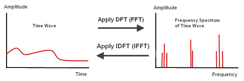
Diagram 1

The equation for the Discrete Fourier Transform is: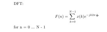

Equation 1

Where F(n) is the amplitude at the frequency, n, and N is the number of discrete samples taken.

Outline For Learning About The DFT and FFT

<< Previous Next >>

Here is an outline of the steps used to explain both the DFT and FFT.

1. First the DFT will be explained. This is the vital first step, since an FFT is a DFT and there are, therefore, basic concepts in common with both. Learning this first will make understanding the FFT easier.
2. Once you understand the basic concepts of a DFT, the FFT will be explained. This is broken into several steps.
3. The "Danielson-Lanczos Lemma" will be explained, which is the first step to understanding the FFT.
4. The "twiddle factor" will be explained, which is another key to understanding the FFT.
5. The "Butterfly Diagram" will be explained. The Butterfly is an FFT in diagram form. It's the final step of this tutorial and builds on the prior concepts.
6. Several examples will be given along with the basic concepts above.

The Goal of This Tutorial

<< Previous Next >>

The goal of this tutorial is to show how to take a discretely sampled wave, usually from nature, and convert it to the frequency domain by using an FFT. An FFT is a DFT of a particular form. An FFT is simply a fast way of calculating a DFT. Before explaining the FFT I explain the DFT. I do this for three reasons.

1. A DFT is much simpler to understand mathematically, which is better for learning.
2. Once you understand what the terms of a DFT mean, they apply to the FFT, so you are learning the FFT too.
3. You will gain an appreciation for what the FFT accomplishes, because it is derived from the DFT and the only purpose of the complex math of an FFT is to speed up the DFT calculation. It's purely about speedy number crunching and changes none of the fundamentals.

Why Do This?

<< Previous Next >>

The reason to learn about the DFT and FFT is in order to get a frequency spectrum of a wave or to understand better what frequencies it is composed of. This might allow you to better identify, for example, a sound wave that you have sampled than could be done with the time wave, which is useful for speech recognition. Or, maybe you want to add or subtract frequencies and recreate the original wave with these modifications using an inverse Fourier Transform. Doing this with light waves you could, for example, remove dirty spots or noise from an image, or find recurring patterns in an image. You may have other ideas as to what you can do with the frequency components of a wave. The sky is the limit!

The DFT

<< Previous Next >>

The Discrete Fourier Transform converts discrete data from a time wave into a frequency spectrum. Using the DFT implies that the finite segment that is analyzed is one period of an infinitely extended periodic signal.

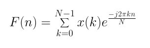
The DFT equation:

Equation 1

x(k) is the time wave that is converted to a frequency spectrum by the DFT.

Here are key concepts required to understand a DFT:

1. The "sampling rate", sr. The sampling rate is the number of samples taken over a time period. For simplicity we will make the time interval between samples equal. This is the "sample interval", si.
2. The fundamental period, T, is the period of all the samples taken. This is also called the "window".
3. The "fundamental frequency" is f0, which is 1/T. f0 is the first harmonic, the second harmonic is 2*f0, the third is 3*f0, etc.
4. The number of samples is N.
5. The "Nyquist Frequency", fc, is half the sampling rate. The Nyquist frequency is the maximum frequency that can be detected for a given sampling rate. This is because in order to measure a wave you need at least two sample points to identify it (trough and peak).
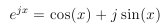
6. "Euler's formula" -- 
7. The sampled part of the time wave, x(t), should be "typical" of how the wave behaves over all time that it exists.
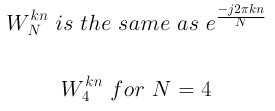
8.  This notation makes handling the exponential easier. This is sometimes called the "twiddle factor."

For simplicity, we will sample a sine wave with a small number of points, N, and perform a DFT on it, then we will employ each of the concepts above. Note, the sine wave is a time wave, and could be any wave in nature, for example a sound wave. The horizontal axis is time. The vertical axis is amplitude.

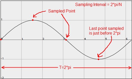
Diagram 1

Notice how in the diagram above we are sampling four points. The fundamental period, T, of the wave sampled is set to 2*pi. This applies to any wave we want to sample. The interval between samples is 2*pi/N, so in this case it is 2*pi/4. Thus, the interval between samples is pi/2 in this case.

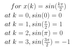
The time wave is thus, x(k) = sin(pi/2*k) for k = 0 to N -1. The last point sampled is always the point just before 2*pi, because the wave is considered to be a repeating pattern and wraps around back to the value at k = 0, so you aren't missing any information.

We also need to know the time taken to sample the wave, so that we can tie it to a frequency. In our example, the time taken for the fundamental period, T, is 0.1 seconds (this value is measured when the wave is captured). That means the sine wave is a 10 Hz wave. Hertz = cycles per second. Also, the sampling interval, si, is the fundamental period time divided by the number of samples. So, si = T/N = 0.1/4 seconds, or 0.025 seconds. The sampling rate, or frequency, sr, = 1/si = 40 Hz, or 40 samples per second.

For the sine wave, the value at each of the four points sampled is:

And, before we plug into the DFT, some more on Wn, the twiddle factor, referenced above:

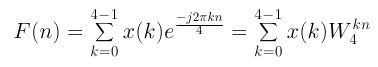
The DFT formula, then, for a four point sample and with the twiddle factor is:

Now, Euler's Formula for N=4:

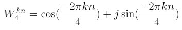
Equation 2

For the equation above, where k*n = 0 to N - 1, i.e. 0 to 3, here are the results:

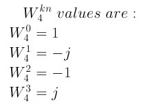
Notice that any additional integer values of kn will cycle back around. For example, kn = 4 cycles back to kn=0, so the value is 1. kn = 5 cycles back around to kn = 1, so the value is -j. The equation "kn modulus 4" determines which value of W is selected. Also, note that for larger samples the cycle is bigger. So for N=8 the equation would be "kn modulus 8". This is probably why W is called the "twiddle factor".

Now put this together for the DFT:

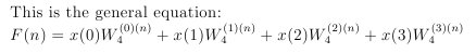
Here is the DFT worked out for all four points and for four frequencies:

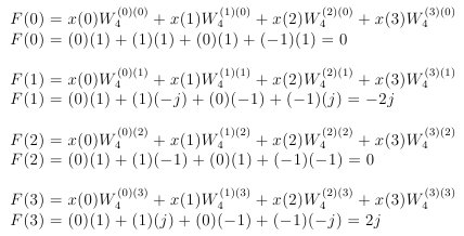
Evaluating the output data. Each F(n) value refers to a particular frequency. The frequency of the point is determined by the fundamental frequency multiplied by n i.e. f = f0*n, where f0=1/T = 10Hz. The output values are the phase of the frequencies, which are represented by a real part and an imaginary part thus: real + j*imaginary. The fundamental frequency, first harmonic, is 10 Hz as calculated above. The magnitude at a frequency is Calculated thus sqrt(real*real + imaginary*imaginary).

Below is a frequency spectrum plot for the sine wave determined from the DFT we just worked through:

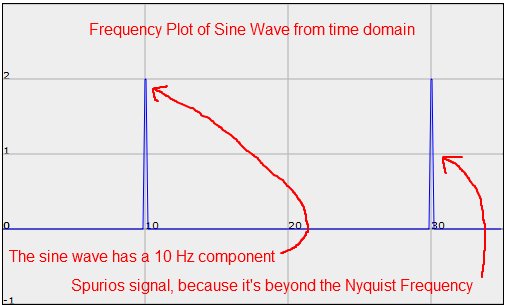
Diagram 2

The frequency plot is in the "frequency domain". The spike at 10 Hz shows that the DFT pulled out one of the frequencies that is in the sine wave. In fact, the sine wave is a 10 Hz sine wave, so that makes sense. However, the spike at 30 Hz should not be there, because there is no 30 Hz wave in the sine wave. So what accounts for that spike? Well, this is where the Nyquist Frequency, fc, mentioned above comes in. The Nyquist frequency is the cut off point above which the data from the DFT is no longer valid. The sampling rate is 40 Hz, and fc is half the sampling frequency, which means that any frequency above 20 Hz will not be valid in this case. So, the 30 Hz frequency is a spurious signal.

That completes analysis of a very simple wave.

Most waves will have many more frequencies in them, and thus many more spikes of various magnitudes along the frequency spectrum. For example, below is a triangle wave in time and the corresponding frequency spectrum of that wave:

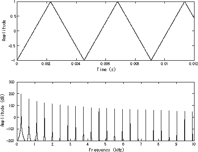
Diagram 3

The Next section is FFT. The FFT builds on the knowledge above, so it should be understood before moving on to the FFT.

Overview of The FFT

<< Previous Next >>

This is a "decimation in time" FFT, because the input value to the FFT is the time wave, x(t). The time wave could be a sound wave, for example.

Speed!

The only reason to learn the FFT is for speed. An FFT is a very efficient DFT calculating algorithm.

How fast is an FFT versus a "straight" DFT?

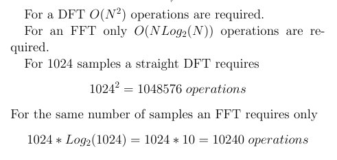
Equation 1

This means that a 1024 sample FFT is 102.4 times faster than the "straight" DFT. For larger numbers of samples the speed advantage improves. For example, for 4096 samples the FFT is over 340 times faster.

x(k) is the time wave that is converted to a frequency spectrum by the DFT.

Learning the FFT is a bit of a challenge, but I'm hoping this tutorial will make it relatively easy to learn. Here is a basic outline of the tutorial:

1. First, you'll need to learn the "Danielson-Lanczos Lemma" (D-L Lemma). This will require long equation writing, but it's a vital component of the FFT. I'll give several examples.
2. You'll need to understand the "twiddle factor" -- . This was discussed a little during the DFT tutorial. It along with the "D-L Lemma" are essential to understanding how an FFT works.
3. Then the "Butterfly Diagram" will be explained. This builds on the first two concepts above. The Butterfly diagram is a diagrammatic representation of an FFT algorithm.
4. You'll also learn about the "reverse bit pattern" for data input and the reason for it.

The Danielson-Lanczos Lemma

<< Previous Next >>

This is the first key to understanding the FFT. It takes quite a few steps, but I've broken the tutorial down into small digestible steps to make this as smooth as possible.

Here is the Danielson-Lanczos Lemma:

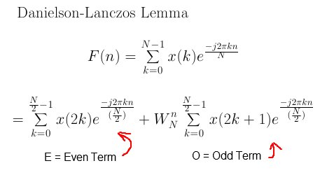
Equation 2

Note it is a DFT broken up into two summations of half the size of the original. The first summation is the "even terms", E, and the second is the "odd terms", O. W is the "twiddle factor", and understanding it is another key to understanding the FFT. Here is the "twiddle factor".

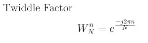
Equation 3

How to Expand the DFT

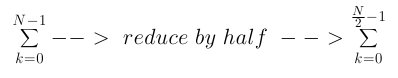
To expand the DFT into even and odd terms as in the lemma above, you do the following. For the even term you substitute 2k into k, then you create a summation of half the size of the original. For the odd term you substitute 2k + 1 into k, then create a summation of half the size of the original.

Here is a the summation halved:

The example below shows the process required for a first level expansion.

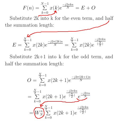
Equation 4

Note the "twiddle factor" above and where it comes from.

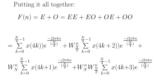
And putting the even and odd terms together from above, we get the Danielson Lanczos first level expansion:

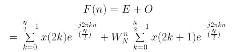
Equation 5

The above is a first level break down. You can continue to break each term down into even and odd terms until you run out of samples and only have one value in the summation. Like this:

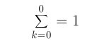
Equation 6

This happens because you keep halving the number of values summed on each expansion of the equation.For the FFT we want all summations to be expanded down to 1 term. Here is the pattern of expansion for the Danielson-Lanczos Lemma:

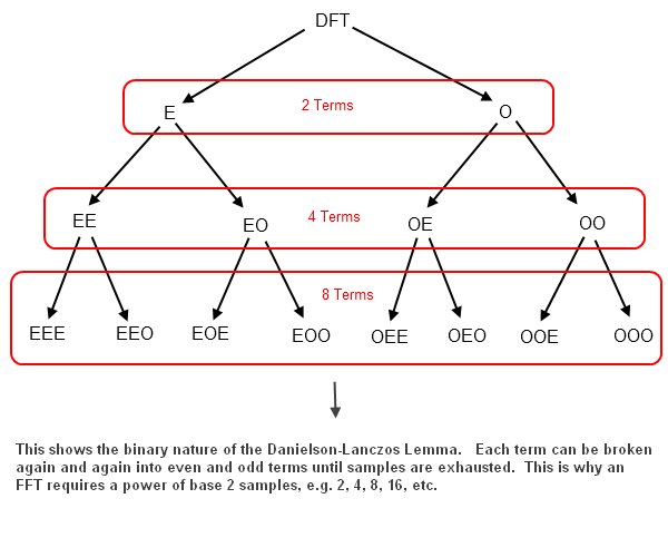
As shown in the diagram above, the D-L Lemma breaks down in a binary manner. That is, the number of terms expands as follows 1, 2, 4, 8, 16, 32, etc. In order to get all of the summation to unity, 1, therefore, we must have a power of base 2 number of samples, or N=2^r samples. So, an FFT requires N = 2^r samples.

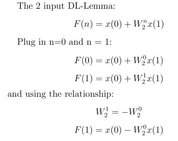
For a sample size of N=2, a first level expansion will be enough to get the summations to unity. The first level expansion will look like this after plugging into equation 5 above.

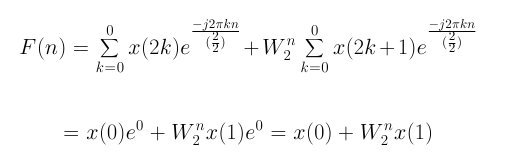
Equation 7

The summations are reduced to unity, and all that remains is a twiddle factor and input values, x(0) and x(1). This is the general form used for the Butterfly diagram, shown later in this tutorial.

Next example will be expansion of the D-L Lemma to 4 terms.

Expansion of the Danielson-Lanczos to Four Terms

<< Previous Next >>

For N = 4 samples, the equation must be expanded again to four terms. Below is the expansion to four terms. As with the first level expansion, substitute 2k into k and reduce the summation by half for the even terms and substitute 2k+1 into k and reduce the summation by half for the odd terms. The E and O below refer to equation 5.

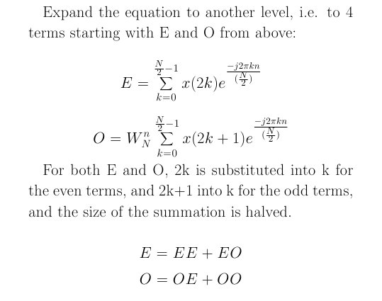
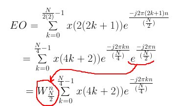
Here is the even value expanded from E:

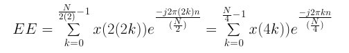
Here is the odd value expanded from E:

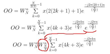
Here is the even value expanded form O:

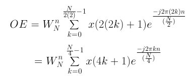
Here is the odd value expanded from O:
.

And finally:

Equation 8

Now, N = 4 samples, and using the same procedure as was used for two samples, equation 8 becomes:

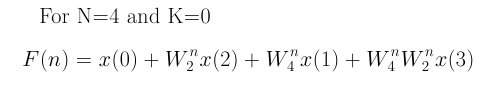
Equation 9

Once again, as with N=2, the summations have been reduced to unity, and all you have remaining are "twiddle factors" and the input values, x(0), x(1), x(2), and x(3).

The next example will be an 8 term expansion, shown but not worked through.

The Danielson-Lanczos Lemma Expanded to 8 Terms

<< Previous Next >>

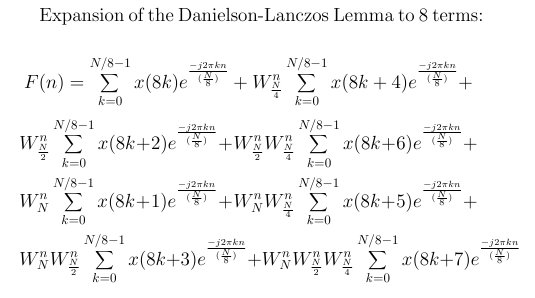
Equation 10

After the expansion above you can plug in for N = 8 samples, and k=0, since all summation would be unity when N=8.

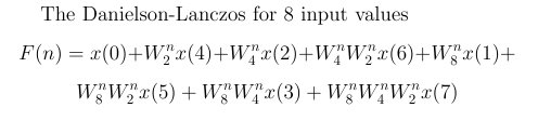
Equation 11

Danielson-Lanczos Lemma Observations

<< Previous Next >>

Note two things about the equations 7, 9 and 11, repeated below. First, the order of input values, x(n), is "reverse binary".For example, left to right the order for the 4 term equation is x(0), x(2), x(1) and x(3). The order for the 8 term equation is x(0), x(4), x(2), x(6), x(1), x(5), x(3), and x(7). This naturally happens when the D-L Lemma is expanded. The Butterfly Diagram makes use of this fact. The second thing to note is that the "twiddled factors",W, build up with each new expansion, so that you multiply more together. The Butterfly diagram also deals with this by the adding of "stages", which you will see later in this tutorial.

Equation 7

Equation 9

Equation 11

More on the "Reverse Binary" pattern.

Here are two examples of the "reverse binary" example:

For 4 inputs:

Count from 0 to 3 in binary 00, 01, 10, 11. Now, reverse the bits of each number and you get 00, 10, 01, 11. In decimal this is 0, 2, 1, and 3.

So, the values in the D-L equation would be x(0), x(2), x(1), and x(3). This is what you see in equation 9 above.

For 8 inputs:

Count from 0 to 7 in binary 000, 001, 010, 011, 100, 101, 110, 111. Now, reverse the bits of each number and you get 000, 100, 010, 110, 001, 101, 011, 111. In decimal this sequence is 0, 4, 2, 6, 1, 5, 3, and 7.

So, the values in the D-L equation for 8 samples would be x(0), x(4), x(2), x(6), x(1), x(5), x(3), and x(7). This is what you see in equation 11 above.

The same pattern holds for all expansions of the D-L Lemma, and is made use of by the Butterfly Diagram.

Next I'll discuss the "twiddle factor" and then put it together with the Danielson-Lanczos Lemma to create the Butterfly diagram, which is the FFT in diagram form.

The "Twiddle Factor"

<< Previous Next >>

The twiddle factor, W, describes a "rotating vector", which rotates in increments according to the number of samples, N. Here are graphs where N = 2, 4 and 8 samples.

c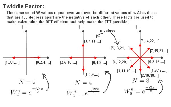

The Redundancy and Symmetry of the "Twiddle Factor"

As shown in the diagram above, the twiddle factor has redundancy in values as the vector rotates around. For example W for N=2, is the same for n = 0, 2, 4, 6, etc. And W for N=8 is the same for n = 3, 11, 19, 27, etc.

Also, the symmetry is the fact that values that are 180 degrees out of phase are the negative of each other. So for example, W for N =4 samples, where n = 0,4,8, etc, are the negative of n = 2,6,10, etc.

The Butterfly diagram takes advantage of this redundancy and symmetry, which is part of what makes the FFT possible.

The Butterfly Diagram

<< Previous Next >>

The Butterfly Diagram builds on the Danielson-Lanczos Lemma and the twiddle factor to create an efficient algorithm. The Butterfly Diagram is the FFT algorithm represented as a diagram.

First, here is the simplest butterfly. It's the basic unit, consisting of just two inputs and two outputs.

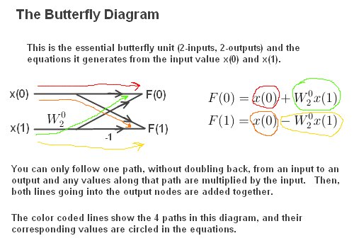
That diagram is the fundamental building block of a butterfly. It has two input values, or N=2 samples, x(0) and x(1), and results in two output values F(0) and F(1). The diagram comes form the D-L Lemma for two inputs.

This can be shown by taking equation 7 above and plugging in for values n=0 and n=1, thus:

So, the Butterfly comes from the Danielson-Lanczos Lemma, but it also uses the twiddle factor to take advantage of redundancies and symmetry in the D-L Lemma.

To get a full understanding of the Butterfly, a four input Butterfly will be required. That is described next.

Constructing A 4 Input Butterfly Diagram

<< Previous Next >>

Here I will show you step-by-step how to construct a 4 input Butterfly Diagram.

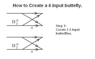
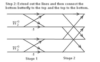
Next extend lines and connect upper and lower butterflies.

Finally, labeling the butterfly.

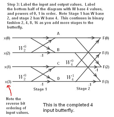
Note the order of input values is "reverse bit" order. The Butterfly uses the natural expansion order of the Danielson-Lanczos Lemma, which is why the input is ordered that way. This was described earlier.

The four output equations for the butterfly are derived below.

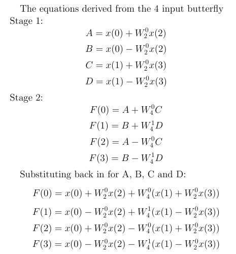
Equation 12

The N Log N savings

Remember, for a straight DFT you needed N*N multiplies. The N Log N savings comes from the fact that there are two multiplies per Butterfly. In the 4 input diagram above, there are 4 butterflies. so, there are a total of 4*2 = 8 multiplies. 4 Log(4) = 8. This is how you get the computational savings in the FFT! The log is base 2, as described earlier. See equation 1.

In the next part I provide an 8 input butterfly example for completeness.

An 8 Input Butterfly

<< Previous Next >>

Here is an example of an 8 input butterfly:

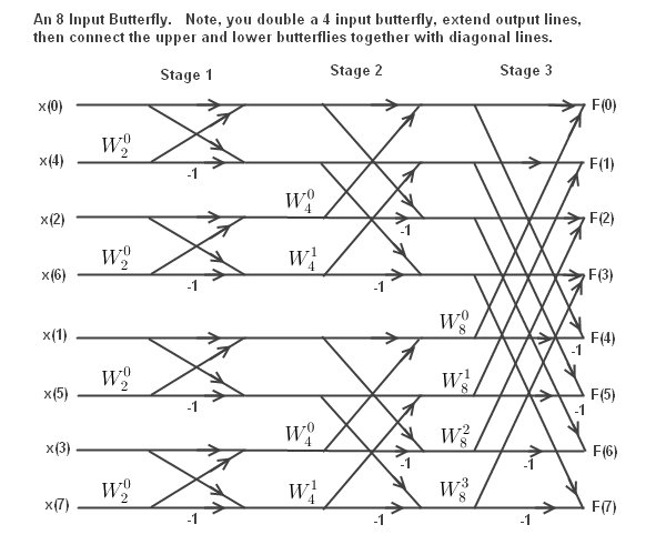
An The 8 input butterfly diagram has 12 2-input butterflies and thus 12*2 = 24 multiplies.

N Log N = 8 Log (8) = 24. A straight DFT has N*N multiplies, or 8*8 = 64 multiplies. That's a pretty good savings for a small sample. The savings are over 100 times for N = 1024, and this increases as the number of samples increases.

You can keep expanding the butterfly by the same procedure.